Types of Points

For a lot of GIS-technicians points come in very handy in representing a diversity of issues. Lanterns and road signs are easily represented as points in GIS. Hill peaks, trees, badger setts and observations of animals can be handled as points as well. In transportation the locations of ships, trucks or emergency vehicles are tracked by means of GPS where the data are measured and stored as points with two coordinates defined.

Obviously a variety of things are handled by the same representational feature class. In a mathematical sense points are zero dimensional objects with no extent. In all of the cases above this means that the original elements are reduced until their size converges to zero. This representational 'equifinality' of all these objects might mislead to the temptation that they could be analyzed in a similar way. In the following I will try to clarify the reasons and properties why this is not the case.

There are many ways to approach a classification of point data. In this work I will distinguish the four following aspects often implicitly or explicitly inherent to a point object in a GIS:

1.	Generator/Generation Mechanism
2.	Object type
3.	Sampling method
4.	Representation

Researchers often wish to know the generation mechanism which created a certain spatial pattern found. This mechanism is most often unknown and can often only be inferred from the resulting patterns. Since it is seldom known in advance, there is not much use in classifying point objects upon this first aspect.

The second aspect can be clarified by asking the following two questions:

2a.	Does a single object change its location?
2b.	How long does the object exist?

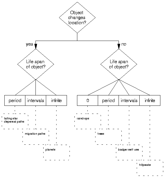
The ordering of the questions does not really matter. Figure 2.1 illustrates the two questions and a possible classification scheme. The distinction between moving and static objects seems to be trivial but is nonetheless important as can be seen below. The question on the life span of an object splits up several types. Objects that only exist for a fraction of a second can be distinguished from ones that exist for a longer time, for multiple times or even infinitely. Objects that change their location cannot have a life span of 0, because they must exist at least at two different locations which for zero dimensional objects requires the existence at two different times.

Cressie (1993) only considers temporal point objects which do not change their location. He distinguishes only two types. They are called space-time shock point processes and space-time survival point processes. For the first type, events occur instantaneously over both time and space. Conversely, for the latter type, events are born at some random location and time, and then live for a random length of time. These are the only temporal point patterns considered by Cressie (1993). The other types of point objects considered here (figure 2.1) were missing, probably due to the fact that his work is concentrating on examples originating from the field of botany.

In the present work I will concentrate on objects that change their location and exist for a certain period of time.

One of the factors which is often 'hiding' the type of object is the sampling scheme applied when collecting data (figure 2.2). For example in wildlife telemetry locations of animals are often taken at certain intervals such as days or weeks. They are then recorded as point objects with two coordinates and a time identifier. In a subsequent analysis they are often considered in an equal manner as if they were objects existing only at the observed locations. The locations in between samples are ignored even though the animal must have passed some of the area between the samples.

Figure 2.1: Classification of Point types.

The sampling scheme needs to define at least three aspects which can be evaluated by the following three questions:

1.	What is the temporal sampling scheme?
2.	What is the spatial sampling scheme?
3.	What kind of boundary is defining the sampling area? (infinite/none, bordered)

The temporal sampling scheme is of concern here. When applying different schemes (figure 2.2) the resulting data and their representation is changed accordingly. In the past most of the data in spatial studies on animals were applying some kind of a snapshot sampling scheme. This resulted in data sizes which could still be handled. The researchers were mostly concerned about temporal autocorrelation of the data in order to be able to apply certain statistics that require independence among observations. They almost never considered the accurate description of an animal's movement as a matter of interest (e.g., White and Garrot, 1990), although such an approach seems to be reasonable in the case of moving objects. We might need to apply a so-called lateral thinking (de Bono, 1972) to overcome these limitations and start developing new analytical methods.

Figure 2.2: Classification of temporal sampling schemes.

It is difficult to judge whether the available statistical methods required the sampling scheme outlined above or that the sampling methods used stimulated the development of the statistical methods. Anyhow, the fact is that today's analytical methods for spatial point objects concentrate on snapshot oriented temporal sampling schemes. Most if not all of them ignore the temporal domain and hence make no distinction between the analysis of static and mobile objects. Even in newer text books on spatial statistics (e.g., Arlinghaus, 1996) chapters on sampling methods completely neglect the need for defining temporal sampling schemes, obviously due to the fact that no established methods for analyzing such data exist.

We need to break up this interdependence of development of analytical methods according to the available data and vice versa sampling data according to the available statistical methods.