Point Pattern Analysis in Biology

Compared to the literature on point pattern analysis in GIS (see below), a larger variety of methods is used in the biological and especially in the ecological literature. Several simple descriptive measurements have been used to describe aspects of point distributions. The easiest of them is probably the mean center, which is easily calculated as:

$$\bar{X} = \frac{\sum X_i}{N} , \bar{Y} = \frac{\sum Y_i}{N}$$ (3.1)

N = number of points
$\bar{X},\bar{Y}$ = mean of X and Y

Since the mean center as calculated above is heavily influenced by outliers in the data, the median center is often considered to be a better method to describe a central locality.

The median center is described in two different ways. Cole and King (1968) and Hammond and McCullagh (1978) define the median center analogously to the one dimensional case as the intersection point for the separate medians in the x and y directions. This definition has the problem that the median center depends on the layout of the coordinate system. Rotating the coordinate system results in a different location for the median center. In contrast, Neft (1966), King (1962) and Smith (1975) define it as the point, where the sum of distances to all points is at a minimum (minimum aggregate travel). The point is calculated in an iterative process using successively finer grained grids.

Among the most commonly used easier measurements of spread in point data is the standard distance. The standard distance used in geostatistics is analogous to the standard deviation in simple, descriptive statistics. It can be calculated as:

$$SD = \sqrt{\frac{ \sum (X_i - \bar{X})^2}{N} + \frac{ \sum(Y_i - \bar{Y})^2}{N}}$$ (3.2)

which can be rewritten for faster computation as:

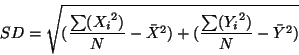$$SD = \sqrt{(\frac{\sum ({X_i}^2)}{N} - \bar{X}^2) + (\frac{\sum ({Y_i}^2)}{N} - \bar{Y}^2)}$$ (3.3)

SD = standard distance
N = number of points
$\bar{X},\bar{Y}$ = mean of X and Y

Since the standard distance uses squared distances, it exaggerates the importance of extreme points. In a more spatially explicit way a measurement of spread of points can be achieved by calculating the standard deviational ellipse.

Traditionally, quadrat-density analysis and nearest neighbor methods have been widely used (Carpenter and Chaney, 1983; Legrendre and Fortin, 1989) in biology to assess the deviation from complete spatial randomness.

There are two ways to check for random patterns by quadrat counts using the Poisson distribution as a reference:

• compare the actual quadrat counts to the expected distribution
• use the variance-mean ratio of the observed distribution

To compare the observed quadrat counts to a Poisson distribution expected under the hypothesis of complete spatial randomness, a $\chi^2$ statistic can be calculated as follows:

$$\chi^2 = \sum{\frac{(X_i - \bar{X})^2}{\bar{X}}}$$ (3.4)

X_i = number of points in each quadrat
$\bar{X}$ = mean number of points per quadrat

with N - 1 degrees of freedom.

The Poisson distribution has a variance equal to the mean, thus departures from unity in the ratio reflect tendencies towards either clustering or regularity. The degree of departure from 1 can be converted to a z score after calculating the standard error of the difference (SE_x) from:

$$SE_x = \sqrt{\frac{2}{N-1}}$$ (3.5)

$$z = \frac{observed\ ratio - expected\ ratio}{SE_x}$$ (3.6)

N = total number of quadrats

Several indices for quadrat count data have been developed. An overview can be found in table 3.1.

Table 3.1: Indices for Quadrat Count Data (after Cressie (1993)).

Name	Index	Reference
Relative variance	I	Fisher et al. (1922)
David-Moore index	ICS	David and Moore (1954)
Index of Cluster Frequency	ICF	Douglas (1975)
Mean Crowding	X	Lloyd (1967)
Index of Patchiness	IP	Lloyd (1967)
Morisita's Index	$I_{\delta}$	Morisita (1959)
(Xingping)	La	Xingping (1996)

These quadrat count methods have been enhanced for overcoming their dependency of scale by selecting a certain quadrat size. Greig-Smith (1952) basically proposed a resampling to successively coarser grid sizes using $\chi^2$ statistics. Mead (1974) uses another approach using successively coarser blocks of 4 x 4 subblocks and testing the set of counts against a random selection from (16!)/(4!)⁵ = 2627265 possibilities, as implied by complete spatial randomness.

Apart from the methods based on quadrat counts, a second family of analysis methods is widely used in the study of point patterns. One of the earliest methods available is the nearest neighbor distance.

Evans and Evans (1954) developed a measurement index and linked it to the Poisson probability distribution. The analysis compares an observed spacing of a point distribution to an expected random pattern. The average expected distances for a random pattern are calculated as:

$$\bar{r}_e = 0.5 * \sqrt{\frac{A}{N}}$$ (3.7)

$\bar{r}_e$ = average expected distance
A = area of study region
N = number of points

The above formula is intended for use with a study area without border effects. If the study area has border effects, the above formula underestimates the expected average nearest neighbor distance for a random pattern. As this is a common source of error, I will shortly illustrate this effect in the following paragraphs.

As an example the average nearest neighbor distance from 1000 random simulations is 158 meters for the badger setts data from Good (1997) for the Sihlwald area, whereas the above formula results in 144 meters. Considering only the 35 large setts (with more than 3 entrances) the corresponding values are 314 and 270 meters respectively.

There are two approaches to cope with these border effects. One can construct an outer edge of the study area where points lying inside this edge area are only used for distance calculations for points lying in the inner (kernel) area, but are not taken as observations. An other approach is to perform Monte Carlo simulations by generating random points within the study area and then calculating the nearest neighbor distances for each simulation. The advantage of this method is that one can use all observations in the calculations. The disadvantage is the large amount of computing time needed. Since biological data analyzed with nearest neighbor methods are often based on scarce samples, it is desirable to use all data available.

Figure 3.1: Effect of shape of the study area on the expected average nearest neighbor distance. Calculations made from simulations of random patterns.

The effect of shape of the study area on the average nearest neighbor distance in a random distribution is illustrated in figure 3.1. The six shapes all have an area of 16 hectares. In each shape the mean nearest neighbor distance was approximated by simulations for 20, 50, 100 and 200 random points. Two results can be deduced from figure 3.1: (1) The mean nearest neighbor distance for random samples increases with an increase of the border effects. (2) This effect is stronger for smaller sample sizes.

The expected distance for a (maximally) dispersed pattern is given by:

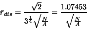$$\bar{r}_{dis} = \frac{\sqrt{2}}{3^{\frac{1}{4}}\sqrt{\frac{N}{A}}} = \frac{1.07453}{\sqrt{\frac{N}{A}}}$$ (3.8)

$\bar{r}_{dis}$ = expected distance
A = area of study region
N = number of points

To test the significance of patterns, Getis (1964) used the standard error of the expected average nearest neighbor distance to calculate a z value. The average expected distances for nth-order neighbor distances can be calculated as:

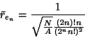$$\bar{r}_{e_n} = \frac{1}{\sqrt{\frac{N}{A}}\frac{(2n)!n}{(2^{n}n!)^2}}$$ (3.9)

$\bar{r}_{e_n}$ = average expected distance to the nth neighbor
n = order of nearest neighbor
N = number of points
A = area of study region

These methods using distances have been enhanced for cases where measurements are taken from observation points to the events of interest (Doguwa and Upton, 1989; Diggle, 1983).

With the exception of the order neighbor distances, the above methods are also of limited use due to their inability to work over a range of scales. This difficulty has been addressed by several authors and resulted in the development of second-order functions (e.g., K-, L- and G-functions), which became more and more popular (Getis, 1984; Moutka and Penttinen, 1994; Tomppo, 1986; Ripley, 1988; Getis and Franklin, 1987). For these functions some methods for edge effect corrections have been published (e.g., Haase, 1995; Doguwa and Upton, 1989).

As another area of interest, different methods for density estimation are available. The earliest methods were simply counting the number of quadrats in which observations were found. Today a variety of methods are in use ranging from Dirichlet tessellations, least diagonal neighbor tessellations, weighted triangles and weighted polygons (Upton and Fingleton, 1985) to complex kernel estimations, harmonic mean methods and Bayesian smoothing (Dixon and Chapman, 1980; Worton, 1989). These methods are being widely used in wildlife research to gain more information from the observations than is possible using traditional homerange analysis methods such as the convex polygon.

Perry and Hewitt (1991) introduced a new class of tests for spatial patterns referred to as SADIE (Spatial Analysis by Distance Indices). They compare the spatial arrangement of the observed sample with other arrangements derived from it, such as those where the individuals are crowded or as regularly spaced as possible. Perry (1995) extends the method for two-dimensional patterns using Voronoi tessellations which are iteratively transformed into a regular pattern.

Area estimation for example in homerange analysis has also received special attention especially in wildlife research, and over a dozen methods have been used (e.g., Dixon and Chapman, 1980; Samuel and Garton, 1985; White and Garrot, 1990; Worton, 1989).

In recent years, surface pattern analysis methods such as Moran's I, Geary's c, correlograms, (semi-) variograms and two-dimensional spectral analysis appeared frequently in the biological literature (Legrendre and Fortin, 1989; Renshaw and Ford, 1984). These methods are often used with aggregated data representing surfaces rather than point patterns.

Andersen (1992) used Ripley's K-function (Ripley, 1976) for interaction models using 'static' point pattern data. He expresses the need for statistical methods that explicitly allow for both spatial and temporal structure. Knox's method (Knox, 1964) for analyzing space-time interactions using 2-way tables is problematic because of the assumed independence of events (O'Kelly, 1994). O'Kelly (1994) presents a new approach using clustering techniques which allow for interdependence between the clusters.

Biondini et al. (1988) presented a new technique for analyzing multivariate patterns using permutation procedures. It has been applied to zoological point data (White and Garrot, 1990) with promising results for multivariate point patterns. In the zoological literature, habitat analysis is often done using Chi-squared analysis described in Neu et al. (1974) and its various modifications (see White and Garrot, 1990). Other statistical methods such as compositional analysis and log-linear models have also been reported (Heisey, 1985; Aebischer and Robertson, 1993). One of the major problems with these methods is the condition for independence of the observations (Swihart and Slade, 1985; Dunn and Gipson, 1977). Time aspects are only included by separately analyzing different time spans (e.g., Stoms et al., 1993).